Introduction to Spherical Harmonics for Graphics Programmers
published on Apr 12 2026
On your computer graphics journey, you will eventually run into some paper or code mentioning spherical harmonic functions. They are indeed a very useful tool: with just a few coefficients, they allow us to approximate a given function defined on a sphere. This can be very useful for modeling complex lighting.
While spherical harmonics are a very well studied subject, trying to make sense of them can still be a bit intimidating. However, I think that understanding the applications of spherical harmonics in the field of realtime computer graphics need not be that difficult.
In this article, I will try my hand at explaining spherical harmonics the way I wish they had been explained to me. I hope that by the end readers will be ready to digest more advanced technical material that uses or talks about spherical harmonics.
While the reader is expected to have some baseline level of familiarity with realtime rendering, linear algebra and integrals, it's nothing too crazy - we won't be doing any rigorous proofs, and any derivations we'll do are simple basic algebra.
Why Do We Even Care?
Before we start, I guess it should be properly explained why we, as practitioners of computer graphics, are even interested in spherical harmonics.
Any function that associates some quantity/value with a direction in 3D space can be thought of as a function defined on the domain of a unit sphere. Indeed, a "direction" is a unit vector, and the endpoint of that vector is always some point on the surface of a unit sphere centered at the origin. Going forward we will use "function of direction", "function defined on a sphere", and "function defined on the surface of a unit sphere" interchangeably.
It just so happens that any continuous function defined on a sphere can be represented as an infinite weighted sum of some special polynomials. Those polynomials are, in fact, what we call "spherical harmonics". By truncating that sum and making it finite, we can approximate the function in question.
But why is that interesting? Because polynomials are easy to evaluate, and nontrivial functions defined on the domain of a sphere come up in computer graphics all the time.
For example, the radiance $L_i(p, \vec{\omega_i})$ is a function defined on a sphere: it tells us how much light arrives at a point $p$ from a given direction $\vec{\omega_i}$. Cubemaps can be thought of as "tabulated" forms of such a function. Irradiance at a given point can also be thought of as a function of direction (i.e. "how much would the irradiance at a fixed point be, if the surface normal was oriented a particular way").
Being able to approximate a potentially complex lighting environment by just summing up some polynomials is a very appealing proposition. But things other than lighting can be expressed as functions defined on a sphere too.
For example, spherical harmonics can be used to approximate the thickness of a mesh or volume along a given direction at each surface point. Thicknesses approximated this way can be baked out to a texture atlas, and could be used to simulate phenomena like subsurface scattering (I had first heard this idea from my good friend and talented graphics programmer Bagrat Dabaghyan).
So, spherical harmonics can have uses beyond lighting, though in this article we will primarily concentrate on the lighting use case.
Definition of Spherical Harmonic Functions
By now, we are hopefully sufficiently hyped and motivated to learn, so let’s start with some definitions. Once again, I am not going to be super mathematically rigorous - my goal here is to provide just enough detail so that you, the reader, become equipped to read and understand code and papers that make references to spherical harmonics.
Function Space and Its Basis
From linear algebra, we are familiar with the notions of “linear” or “vector” spaces and their “basis”. In order to be able to properly define spherical harmonics, we will need analogous constructions for the world of functions. This video by Kevin Cassel does a good job of explaining them.
To start with, we will think of a set of functions defined on a certain domain as a “space”. Strictly speaking, all of the definitions here require us to mention the domain on which the functions we’re talking about are defined (you will notice that the video linked above does so). However, for our use case, the domain will always be the unit sphere, so we won’t mention it.
In linear algebra, we call a set of vectors $\vec{v_0}, \vec{v_1}, ..., \vec{v_n}$ “linearly independent” if no vector from that set can be written as a linear combination of the other vectors from that set. In other words, for any $\vec{v_i}$, there do not exist coefficients $a_1,...,a_n$ such that $\vec{v_i}=a_0\vec{v_0}+...+a_n\vec{v_n}$.
Similarly, a set of functions $f_0(x), f_1(x), ... , f_n(x)$ is linearly independent if no function from that set can be expressed as a linear combination of the other functions from that set: given any $f_i$, there are no coefficients $a_0, a_1, ..., a_n$ such that $f_i(x) = a_0f_0(x) + ... + a_nf_n(x)$.
In linear algebra, we have the notion of the inner (or dot) product: for a given pair of vectors $\vec{p} = (p_0, p_1, ..., p_n)$ and $\vec{q} = (q_0, q_1, ..., q_n)$, the inner product $\vec{p} \cdot \vec{q}$ is defined as:
$\vec{p} \cdot \vec{q} = \sum_{i=0}^{n}p_iq_i$
For functions $f$ and $g$, their inner product $\langle f,g \rangle$ is defined as the integral of their product over the domain on which the functions are defined:
$\langle f, g \rangle = \int f(\omega)g(\omega) \,d\omega$
Intuitively, if you think of a function as a vector with an infinite number of dimensions, and integration as analogous to summation, the parallel between the two notions of inner product becomes obvious.
Similarly, the norm of a function is the square root of the function’s inner product with itself.
$\left\| f \right\| = \sqrt{\langle f, f \rangle }$
From this, it should be fairly obvious to see what an “orthonormal set of functions” is: it is a set of functions such that the inner product of any function with itself is 1 (that's the normal part), while the inner product with any other function from the set is 0 (that's the ortho part).
For a linear space, an “orthonormal basis” is an orthonormal, linearly independent set of vectors such that any vector in the space can be uniquely expressed as a linear combination of the vectors in the basis.
Similarly, for a space of functions, an “orthonormal basis” is an orthonormal, linearly independent set of functions, such that any function in the space can be uniquely expressed as a linear combination of the basis functions.
However, it is important to point out that for function spaces, the basis set will always be infinite! Once again, if we think of functions as vectors with an infinite number of dimensions, this makes sense: we know that for N-dimensional vector spaces a basis will always contain N elements, so it makes sense that an "infinite dimensional vector space" would have an infinite basis.
Spherical Harmonic Functions
Spherical harmonic functions (or just “spherical harmonics” for short) are an infinite set of special functions defined on the surface of a sphere that form an orthonormal basis for the entire space of continuous functions defined on a sphere.
Take a step back and think about the implications of the above definition. What does it mean? It means that a continuous function defined on the sphere, no matter how complicated or difficult to evaluate, can be expressed as an infinite weighted sum of spherical harmonic functions.
This fact is of immense practical utility - assuming that spherical harmonic functions themselves are simple to evaluate and that an effective procedure for finding the weights/coefficients exists.
As we had already mentioned, spherical harmonic functions are polynomials, so they are, in fact, easy to evaluate. And there does exist a way to find the coefficients, which we shall talk about later.
Okay, this makes sense so far, but we can’t exactly deal with an infinite number of coefficients on a computer. We will have to store a limited number of them. That's fine, we don't mind dealing with approximations. But how many coefficients should we store, and which ones? And what information are we losing by throwing out some coefficients? The answer to that will be given in the next section.
Spherical Harmonic Degree and Order
Before I show you how spherical harmonic functions actually look, we need to talk about how that set of functions is organized.
SH functions are split into numbered groups often called “frequency bands”. Each band has a number $\ell \in {0,1,2,...}$ associated with it. This number is called the "degree" of the functions within the band. The band with degree $\ell$ contains $2\ell+1$ functions. By convention, the functions within a band of degree $\ell$ are indexed from $-\ell$ to $\ell$, and that index is called the “order” of the function.
Side note: I have seen some sources that use "order" to refer to the thing I called "degree" here and "phase" to refer to the thing I called "order". We will NOT be using that terminology, but be aware that it exists and don't get confused!
A spherical harmonic function with degree $\ell$ and order $m$ is usually denoted like $Y_{\ell}^m$
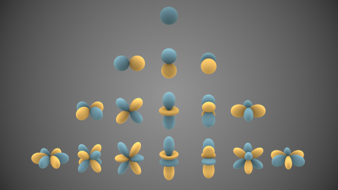
It is instructive to look at a visualization of various spherical harmonic functions sorted by band and order:
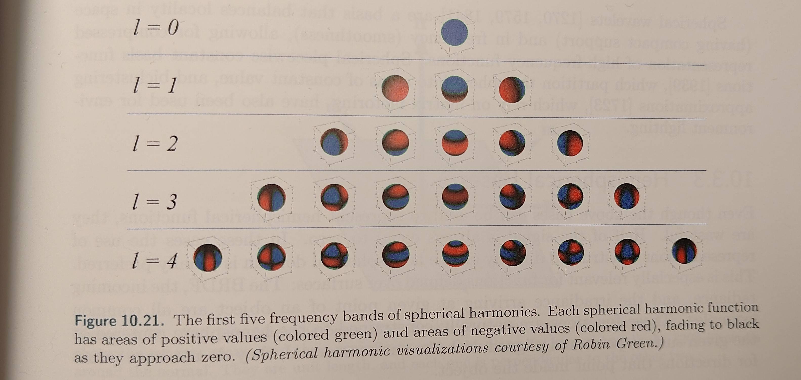 Photo taken from the
Realtime Rendering
book, original visualization by Robin Green. Original used red and green
colors for visualization, this version has been hue-shifted for accesibility
reasons.
Photo taken from the
Realtime Rendering
book, original visualization by Robin Green. Original used red and green
colors for visualization, this version has been hue-shifted for accesibility
reasons.
It can be seen from the illustration above that spherical harmonics with a smaller degree capture larger (or, “low frequency”) details, whereas SH with a larger degree capture smaller (or, “higher frequency”) details.
Recall the question we had posed earlier: what type of information are we losing by truncating the infinite sum? The picture above makes it clear: we lose information about small-scale variations within the function that we're trying to approximate. In other words, we lose detail.
If the function which we are trying to approximate is “low-frequency” (i.e. changes slowly), we should be able to get away with storing coefficients for only the first few bands. For practical applications in realtime computer graphics, we never go beyond bands with single-digit degrees, and moreover, even just degree $\ell=2$ is enough for many applications.
A Look at the Spherical Harmonic Polynomials
So far we’ve only talked about the spherical harmonic functions, but we haven’t seen what they actually look like. We will now take a look at the polynomial forms of spherical harmonic functions within the first three bands, because we'll use those in our upcoming example.
Here is some code that calculates those. It's in JavaScript because our example will be running in the browser.
// Having these constants makes writing down the basis functions easier.
const RECIP_PI = 1/Math.PI;
const C = [
  Math.sqrt(RECIP_PI) * 0.5,
  Math.sqrt(3 * RECIP_PI) * 0.5,
  Math.sqrt(15 * RECIP_PI) * 0.5,
  Math.sqrt(5 * RECIP_PI) * 0.25,
  Math.sqrt(15 * RECIP_PI) * 0.25,
  Math.sqrt(70 * RECIP_PI) * 0.125,
  Math.sqrt(105 * RECIP_PI) * 0.5,
  Math.sqrt(42 * RECIP_PI) * 0.125,
  Math.sqrt(7 * RECIP_PI) * 0.25,
  Math.sqrt(105 * RECIP_PI) * 0.25];

// SH basis functions up to degree l=3.
// Source for SH basis function definitions:
// "Stupid Spherical Harmonics Tricks", Peter-Pike Sloan, 2008
function y00(x,y,z) { return C[0]; }
function y_11(x,y,z) { return C[1] * y; }
function y01(x,y,z) { return C[1] * z; }
function y11(x,y,z) { return C[1] * x; }
function y_22(x,y,z) { return C[2] * y * x; }
function y_12(x,y,z) { return C[2] * y * z; }
function y02(x,y,z) { return C[3] * (3 * z * z - 1.0); }
function y12(x,y,z) { return C[2] * x * z; }
function y22(x,y,z) { return C[4] * (x*x - y*y); }
function y_33(x,y,z) { return C[5] * y * (3*x*x - y*y); }
function y_23(x,y,z) { return C[6] * z * (y*x); }
function y_13(x,y,z) { return C[7] * y * (5*z*z -1); }
function y03(x,y,z) { return C[8] * z * (5*z*z - 3); }
function y13(x,y,z) { return C[7] * x * (5 * z * z - 1); }
function y23(x,y,z) { return C[9] * z * (x*x - y*y); }
function y33(x,y,z) { return C[5] * x * (x*x - 3*y*y); }

// Evaluates SH basis functions with degrees up to and including l for the
// given direction d, returning the result as a Float32 array where each
// element is the value of the corresponding basis function.
// Only supports values of l <= 3.
function evalSHBasis(d, l) {
  const x = d[0];
  const y = d[1];
  const z = d[2];
  switch(l) {
  case 0: return new Float32Array([y00(x,y,z)]);
  case 1: return new Float32Array([
    y00(x,y,z), // l = 0
    y_11(x,y,z), // l = 1
    y01(x,y,z),
    y11(x,y,z)]);
  case 2: return new Float32Array([
    y00(x,y,z), // l = 0
    y_11(x,y,z), // l = 1
    y01(x,y,z),
    y11(x,y,z),
    y_22(x,y,z), // l = 2
    y_12(x,y,z),
    y02(x,y,z),
    y12(x,y,z),
    y22(x,y,z)]);
  default: return new Float32Array([
    y00(x,y,z), // l = 0
    y_11(x,y,z), // l = 1
    y01(x,y,z),
    y11(x,y,z),
    y_22(x,y,z), // l = 2
    y_12(x,y,z),
    y02(x,y,z),
    y12(x,y,z),
    y22(x,y,z),
    y_33(x,y,z), // l = 3
    y_23(x,y,z),
    y_13(x,y,z),
    y03(x,y,z),
    y13(x,y,z),
    y23(x,y,z),
    y33(x,y,z)]);
  }
}
When writing code dealing with spherical harmonics, you will most likely copy-paste the basis functions from somewhere. Making a mistake while doing so (or the source being incorrect in the first place) is a possibility. In fact, this had happened to me while preparing this post.
Luckily, it's not difficult to verify the basis functions that you have. Remember, a fundamental property of the spherical harmonic basis is that it is supposed to be orthonormal: the inner product of any basis function with itself should be one, whereas the inner product of any basis function with any other basis function different from itself should be zero.
These inner products are integrals that are easy to compute numerically using the dumbest Monte-Carlo implementation.
Here is the code that I used to verify the basis functions listed above.
// Helper to multiply SH coefficients by a scalar value.
function mulScalarBySHCoeffs(scalar, coeffs) {
  return coeffs.map(function(c){return scalar*c;});
}

// Helper to add together two packs of SH coefficients.
function addSHCoeffs(coeffs0, coeffs1) {
  return coeffs1.map(function(c,i){
    return c + (coeffs0.length==0 ? 0 : coeffs0[i]);
  });
}

// Uses simple Monte-Carlo integration to verify that the basis functions
// are orthonormal.
function testBasisFunctions() {
  const numSamples = 100000;
  const numBasisFuncs = 16; // we support l up to and including 3, so 16 funcs.

  // innerProducts[i] contains the inner products of the i-th
  // SH basis function with every SH basis function, including itself.
  var innerProducts = [];
  for (var b = 0; b < numBasisFuncs; ++b) {
    // these arrays will be initialized to 0.
    innerProducts.push(new Float32Array(numBasisFuncs));
  }

  for (var s = 0; s < numSamples;) {
    // Generate a random point on a sphere using simple rejection sampling:
    // * Generate a point within the [-1,-1,-1] - [1,1,1] cube;
    // * If the point is inside the unit sphere, normalize and use it;
    // * Otherwise, try again.
    var xr = Math.random()*2.0-1.0;
    var yr = Math.random()*2.0-1.0;
    var zr = Math.random()*2.0-1.0;
    var n = Math.sqrt(xr*xr+yr*yr+zr*zr);
    if (n>1) continue;
    s++;
    var d = new Float32Array([xr/n, yr/n, zr/n]);

    // Evaluate every SH basis function on the generated sample point,
    // compute the partial inner products and add them to the running totals.
    const basisFunctionValues = evalSHBasis(d, 3);
    for (var b = 0; b < numBasisFuncs; ++b) {
      const bv = basisFunctionValues[b];
      const partialInnerProducts =
        basisFunctionValues.map(function(v) { return v * bv; });
      innerProducts[b] = addSHCoeffs(innerProducts[b], partialInnerProducts);
    }
  }

  // Final step in Monte-Carlo integration: multiply by the measure of the
  // integration domain (4pi in the unit sphere case) divided by number of
  // samples.
  for (var b = 0; b < numBasisFuncs; ++b) {
    innerProducts[b] =
      mulScalarBySHCoeffs(4*Math.PI/numSamples, innerProducts[b]);
  }

  // innerProducts[i][j] should be very close to 1 if j==i and very close to 0
  // otherwise.
  console.log(innerProducts);
}
The polynomial functions listed above are quite simple. You could use them directly and never think about the actual mathematical definition of spherical harmonics. However, if you want to deepen your understanding of the subject a bit, it's necessary to dig into how these functions arise. We'll spend the next couple of sections deriving them.
The Definition
Bridging the gap between the mathematical definition of spherical harmonics and the simple code above has always been a pain point for me.
If you look up “spherical harmonic basis functions”, or try some math textbook, you might encounter this scary beast as the definition of the spherical harmonic function of degree $\ell$ and order $m$:
$Y_{\ell}^m(\theta, \varphi) = (-1)^m \sqrt{\frac{(2\ell + 1)}{4\pi} \frac{(\ell - m)!}{(\ell + m)!}} P_{\ell}^m(\cos \theta) e^{im\varphi}$
I will tell you right now that this is not the form that is usually used in computer graphics. However, the form that we do use contains all of the same building blocks. So, we will just pick apart the formula above, examine each piece one-by-one in isolation and get a bit of a handle on this.
First thing to notice about $Y_{\ell}^m(\theta, \varphi)$ is that it is a function defined in terms of spherical coordinates. This makes sense: after all, we are dealing with functions defined on the surface of a sphere. Now is a good time to establish some coordinate system conventions. Doing so is quite important. Different authors might assume different conventions. So, for example, when you're copying and pasting code, you have to be aware of the original convention that was used, and what the target code that you're pasting into assumes.
This is the convention that we shall be using. It is the same as in Green's spherical harmonics paper.
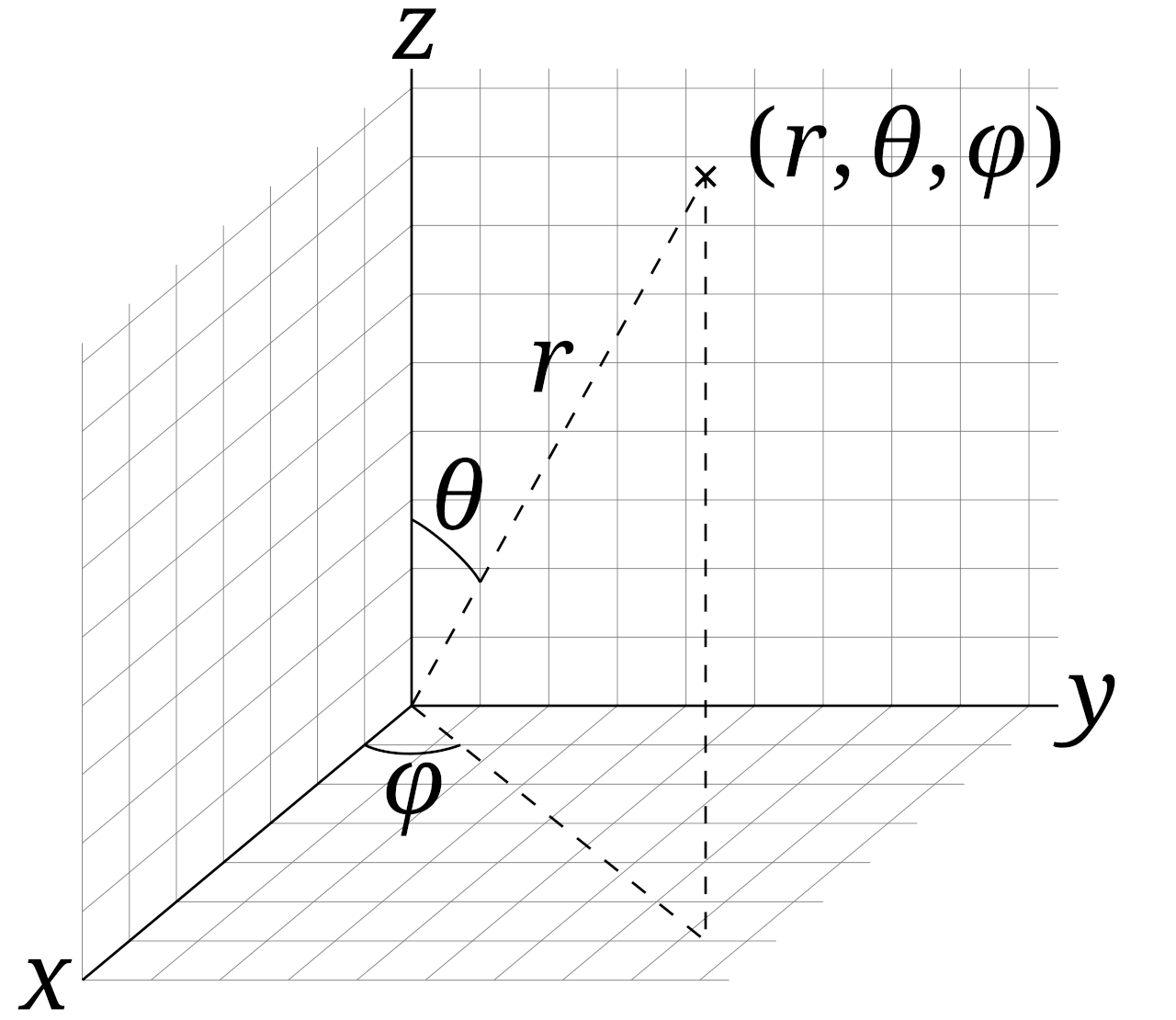
We will assume that the angle $\theta$ is the angle between $Z$ axis and our direction vector and $\phi$ is the angle between the $X$ axis and the projection of our direction vector onto the $XY$ plane. So, the conversion from spherical to Cartesian coordinates is:
| $x =$ | $\cos\phi\sin\theta$ |
| $y =$ | $\sin\phi\sin\theta$ |
| $z =$ | $\cos\theta$ |
With coordinate system stuff out of the way, let's return to our definition. First, we shall deal with this pesky $(-1)^m$ factor. This thing has a fancy name: “Condon-Shortley phase”. We can actually just remove it. In many fields, it is simply ignored and often not even included in the definition. As far as I've seen in computer graphics, it is mostly ignored, though I did see at least one codebase that seemed to include it. But why can we just include or ignore this part as we please?
That question had me stumped the first time I encountered spherical harmonics, but since then I've found an answer that makes sense. Here is my own intuitive understanding of why we can drop the Condon-Shortley phase: spherical harmonics are basis functions. Multiplying them by -1 doesn’t change what can be done with them.
Let’s think back to vectors. In good old 3D the vectors (1,0,0) (0,1,0) (0,0,1) form a basis, but so do the vectors (-1,0,0), (0,1,0) and (0,0,-1). So what if we flipped the sign on some of them? The same logic applies here: the multiplication by -1 doesn’t change the “basisness” or other properties of SH at all: the inner product of the function with itself is still 1, and the inner product of the function with all other functions is still 0. Multiplying by -1 only affects the coefficients needed to represent a given function (similarly to how the same point in 3D space would have different coordinates depending on whether we use left-handed or right-handed coordinate system). For certain applications in physics, having the Condon-Shortley phase is actually important, but for us it will not be relevant going forward. Just be aware that it's a thing, and don't be surprised when you encounter it in the wild.
Next, let’s briefly look at the expression under the square root.
$\sqrt{\frac{(2\ell + 1)}{4\pi} \frac{(\ell - m)!}{(\ell + m)!}}$
It looks unwieldy with the square root and the factorials, but there isn’t much special going on here: ultimately, it’s just a constant needed for normalization (remember, the SH basis is orthonormal). Meaning, if we removed this constant, the inner product $\langle Y_\ell^m, Y_\ell^m \rangle$ would no longer equal 1.
Next, we will examine the mysterious $P_{\ell}^m(\cos \theta)$
This is something called an “associated Legendre polynomial”, or an "associated Legendre function". The $m$ is actually a superscript, not an exponentiation operation!
In the context of spherical harmonic functions, the part containing the associated Legendre polynomial defines how the function changes from pole to pole (because it depends on the polar angle theta).
Formally,
| $P_\ell^m(x) = (1-x^2)^{\frac{m}{2}}\frac{d^m}{dx^m}P_\ell(x)$ | when $m \geq 0$ |
| $P_\ell^m(x) = \frac{(\ell-m)!}{(\ell+m)!}P_\ell^{-m}(x)$ | when $m < 0$ |
Where $P_\ell(x)$ is the Legendre polynomial (the not associated kind), which is given by the formula:
$P_\ell(x) = \frac{1}{2^\ell\ell!}\frac{d^\ell}{dx^\ell}[(x^2-1)^\ell]$
Note that some literature likes to also inject the Condon-Shortley phase into the definition of the associated Legendre polynomial - we do not do this here.
Just for the sake of practice, we can try deriving $P_1^1(x)$:
$P_1(x) = \frac{1}{2}[\frac{d}{dx}(x^2-1)] = \frac{1}{2}(2x) = x$
$P_1^1(x) = \sqrt{(1-x^2)}\frac{d}{dx}P_1(x)=\sqrt{(1-x^2)}\frac{d}{dx}x= \sqrt{(1-x^2)}$
For use in spherical harmonics we substitute $x$ with $\cos\theta$:
$P_1^1(\cos\theta)=\sqrt{1-\cos^2\theta}=\sqrt{\sin^2\theta} = \sin\theta$
You get the idea. We don't actually need to derive every associated Legendre function. The list below should have you covered for pretty much any application in computer graphics:
$ \begin{align*} & P_0^0(\cos \theta) = 1 \\[1ex] & P_1^0(\cos \theta) = \cos \theta \\[1ex] & P_1^1(\cos \theta) = \sin \theta \\[1ex] & P_2^0(\cos \theta) = \frac{1}{2}(3\cos^2 \theta - 1) \\[1ex] & P_2^1(\cos \theta) = 3\cos \theta \sin \theta \\[1ex] & P_2^2(\cos \theta) = 3\sin^2 \theta \\[1ex] & P_3^0(\cos \theta) = \frac{1}{2}(5\cos^3 \theta - 3\cos \theta) \\[1ex] & P_3^1(\cos \theta) = \frac{3}{2}(5\cos^2 \theta - 1) \sin \theta \\[1ex] & P_3^2(\cos \theta) = 15\cos \theta \sin^2 \theta \\[1ex] & P_3^3(\cos \theta) = 15\sin^3 \theta \\[1ex] & P_4^0(\cos \theta) = \frac{1}{8}(35\cos^4 \theta - 30\cos^2 \theta + 3) \\[1ex] & P_4^1(\cos \theta) = \frac{5}{2}(7\cos^3 \theta - 3\cos \theta) \sin \theta \\[1ex] & P_4^2(\cos \theta) = \frac{15}{2}(7\cos^2 \theta - 1) \sin^2 \theta \\[1ex] & P_4^3(\cos \theta) = 105\cos \theta \sin^3 \theta \\[1ex] & P_4^4(\cos \theta) = 105\sin^4 \theta \end{align*} $
There are a few things to note here.
First, don't let the presence of trigonometric functions here confuse you: once we go from spherical coordinates to Cartesian, these will become polynomial functions.
Second, the source for these formulae is the corresponding Wikipedia article, although the version on there also includes the Condon-Shortley phase. I have taken the liberty to remove that here.
Third, you will note that this list only contains entries for positive values of $m$ - it will become clear why later.
One last thing to note is that, as you might have guessed, the "definition" we gave above by far does not tell the whole story. It lacks the larger context about the mathematics that gives rise to these functions, which are the real heart of spherical harmonics.
The associated Legendre functions look the way they do because they're actually solutions to a differential equation called the associated Legendre equation. Unfortunately, describing this equation in detail and solving it goes well beyond the scope of this post. And, of course, you don't actually need to know this part to make use of spherical harmonics in computer graphics.
Still, for those interested, I recommend a series of videos on the topic:
- Legendre Differential Equation and Legendre polynomials
- The Legendre Polynomials in Closed Form
- Rodrigues Formula for Legendre Polynomials (the one we used above to define $P_\ell$)
- Associated Legendre Differential Equation
At last, let’s turn our attention to $e^{im\phi}$. This defines how the SH function behaves with the changing of the azimuthal angle $\phi$. And if you know the famous Euler formula, you’ll know that this equals $\cos(m\phi) + i\sin(m\phi)$ where $i^2 = -1$.
This is the main reason why computer graphics uses a slightly different form of spherical harmonics. The definition we're looking at is actually the definition of complex-valued spherical harmonics: the stuff that can be used to approximate functions that “return” complex numbers. It's very applicable in physics.
But in computer graphics we don’t usually deal with complex-valued functions. Of course, one could simply treat real-valued functions as complex-valued ones where the imaginary part is always zero, but that is not very convenient.
Luckily, there exists a more convenient definition for real-valued functions. Moreover, complex-valued spherical harmonics can be expressed in terms of real-valued ones, and vice versa.
The Actual Definition, for Real This Time
A nice, concise and to-the-point statement of real-valued spherical harmonic functions can be found in this excerpt from Robin Green's paper:
...the SH function is traditionally represented by the symbol $y$:
$ \begin{equation} y_l^m(\theta, \phi) = \begin{cases} \sqrt{2} K_l^m \cos(m\phi) P_l^m(\cos \theta) & \text{if } m > 0, \\ K_l^0 P_l^0(\cos \theta) & \text{if } m = 0, \\ \sqrt{2} K_l^m \sin(-m\phi) P_l^{-m}(\cos \theta) & \text{if } m < 0. \end{cases} \end{equation} $
where $P_l^m$ is the same associated Legendre polynomials we look at earlier and $K_l^m$ is just a scaling factor to normalize the functions: $\begin{equation} K_l^m = \sqrt{\frac{(2l + 1)}{4\pi} \frac{(l - |m|)!}{(l + |m|)!}}, \end{equation}$
This is, with 99.999% certainty, what a computer graphics paper means when it refers to “spherical harmonics”.
This definition also reuses all of the same building blocks that we had looked at in the previous section, so all of this should already be familiar. There are, however, a couple important details to point out.
First, note the normalization constant is different: it uses absolute values of the order $m$. This is in contrast to the definition for the complex-valued case, where the normalization constant uses $m$ directly!
Second, note that we flip the sign of $m$ in the sine and the associated Legendre polynomial in for the $m < 0$ case. This is why the list of associated Legendre polynomials above included only the ones with positive $m$: we don’t need the ones with the negative $m$.
Deriving the Basis Functions
We can now try deriving a few of the basis functions for real-valued spherical harmonics.
Let's start with $y_0^0$. According to the definition cited above, $y_0^0(\theta, \phi) = K_0^0P_0^0(\cos\theta)$.
$K^0_0=\sqrt{\frac{1}{4\pi}}$, which is easy to verify, while $P_0^0(\cos\theta)=1$ according to the table of associated Legendre polynomials cited earlier. Therefore, $y_0^0(\theta, \phi) = \sqrt{\frac{1}{4\pi}}$ - just a constant (also known as a polynomial of 0th degree).
How about $y_{1}^{-1}$? Once again, according to the definition above, $y_{1}^{-1}(\theta, \phi) = \sqrt{2}K_{1}^{-1}\sin\phi P_1^1(\cos\theta)$
$K_1^{-1}=\sqrt{\frac{3}{4\pi}\frac{1}{2}}$, while $P_1^1(\cos\theta)=\sin\theta$.
The square roots of 2 cancel out, so we get: $y_{1}^{-1}(\theta, \phi) = \sqrt{\frac{3}{4\pi}}\sin\phi\sin\theta$
Going from spherical coordinates to Cartesian (using our previously agreed-upon convention), we have $y=\sin\phi\sin\theta$, so the final result in cartesian coordinates is just: $y_{1}^{-1}(x,y,z) = \sqrt{\frac{3}{4\pi}}y$ - so much simpler compared to the formula we started with! Also, note that we changed $\theta, \phi$ to $x,y,z$ in the function parameters, to reflect the coordinate system change.
Using the same exact procedure, it is possible to show that $y_1^0(x,y,z) = \sqrt{\frac{3}{4\pi}}z$ and $y_1^1(x,y,z) = \sqrt{\frac{3}{4\pi}}x$.
As a last example, let's do something slightly trickier: $y_2^2$. Doing simplifications and expanding the associated Legendre polynomial, we get:
$y_2^2(\theta, \phi) = \sqrt{2}\sqrt{\frac{4+1}{\pi} \frac{(2-|2|)!}{(2+|2|)!}}\cos{2\phi}P_2^2(\cos\theta)$ $= \sqrt{\frac{5}{48\pi}}\cos{2\phi}P_2^2(cos\theta)$ $= \sqrt{\frac{5}{48\pi}}\cos{2\phi}3\sin^2\theta$
Let's put this pesky 3 under the square root and simplify further:
$ \sqrt{\frac{5}{48\pi}}\cos{2\phi}3\sin^2\theta = \sqrt{\frac{5*9}{48\pi}}\cos{2\phi}\sin^2\theta = \sqrt{\frac{5*3}{16\pi}}\cos{2\phi}\sin^2\theta = \frac{1}{4}\sqrt{\frac{15}{\pi}}\cos{2\phi}\sin^2\theta $
From trigonometry, we know that $\cos{2\phi}=(2cos^2\phi - 1)$ and that $\sin^2\theta+\cos^2\theta=1$:
$ \frac{1}{4}\sqrt{\frac{15}{\pi}}\cos{2\phi}\sin^2\theta = \frac{1}{4}\sqrt{\frac{15}{\pi}}(2cos^2\phi - 1)\sin^2\theta = \frac{1}{4}\sqrt{\frac{15}{\pi}}(2cos^2\phi\sin^2\theta - \sin^2\theta) = \frac{1}{4}\sqrt{\frac{15}{\pi}}(2cos^2\phi\sin^2\theta - 1 + \cos^2\theta) $
We can now rewrite what we got so far using Cartesian coordinates:
$ \frac{1}{4}\sqrt{\frac{15}{\pi}}(2cos^2\phi\sin^2\theta - 1 + \cos^2\theta) = \frac{1}{4}\sqrt{\frac{15}{\pi}}(2x^2 + z^2 - 1) $
We can make use of the fact that on a unit sphere $x^2+y^2+z^2 = 1$ and clean up the result a bit:
$ \frac{1}{4}\sqrt{\frac{15}{\pi}}(2x^2 + z^2 - x^2 -y^2 -z^2) = \frac{1}{4}\sqrt{\frac{15}{\pi}}(x^2 - y^2) $
So, finally:
$ y_2^2(x,y,z) = \frac{1}{4}\sqrt{\frac{15}{\pi}}(x^2 - y^2) $
Doing this exercise illustrates how we get from the elaborate looking mathematical definition to the simple polynomial forms we had shown earlier in this post. Of course, you don't have to derive them all. There are tables of spherical harmonic functions available. I recommend referring to Appendix A2 of Peter-Pike Sloan's Stupid Spherical Harmonics Tricks paper. It contains SH basis functions in cartesian coordinates for degrees as high as 5 and doesn't have any typos as far as I can tell.
Obtaining the Spherical Harmonic Coefficients
Hopefully at this point we have a general understanding of what spherical harmonics are. We also understand that any piecewise-continuous real-valued function $f(\theta, \phi)$ is representable as an infinite sum:
$f(\theta, \phi) = c_{0}^{0}y_{0}^{0}(\theta,\phi) + c_{1}^{-1}y_{1}^{-1}(\theta,\phi) + c_{1}^{0}y_{1}^{0}(\theta,\phi) + c_{1}^{1}y_{1}^{1}(\theta,\phi) + ...$
where $y_{\ell}^{m}$ are the real-valued spherical harmonic functions, and $c_{\ell}^{m}$ are their corresponding coefficients. The question that we still have to answer is: how do we find those $c_{\ell}{^m}$ coefficients for any given $f(\theta,\phi)$? In other words, how do we go from something like a cube map representation of an image, to a set of SH coefficients that approximates the same thing?
To answer this question, we will look back on our analogy with vector/linear spaces again. Assume we're given some 3D vector $\vec{v}$, and some basis $\vec{i}, \vec{j}, \vec{k}$. How can we compute $\vec{v}$'s coordinates in the frame of reference defined by $\vec{i}, \vec{j}, \vec{k}$?
The answer: we simply have to compute the inner (or dot) products $\vec{v} \cdot \vec{i}, \vec{v} \cdot \vec{j}, \vec{v} \cdot \vec{k}$, which are the lengths of $\vec{v}$'s projection onto $\vec{i}, \vec{j}$ and $\vec{k}$ respectively. In fact, if you recall how a vector is transformed from one coordinate space to another using a matrix, it boils down to nothing more but computing these dot products.
Applying analogous reasoning to the case of functions, in order to compute the coefficient $c_{\ell}^m$, we have to compute the inner product:
$\langle f, y_{\ell}^m\rangle = \int f(\vec{\omega})y_{\ell}^m(\vec{\omega})d\vec{\omega}$
This integral is usually computed numerically, and we'll demonstrate how it can be done in the next section.
Case Study: Projecting a Cubemap onto Spherical Harmonic Basis
Let's start our practical examples with the task of using spherical harmonics to approximate the radiance defined by a cubemap . We will take a small cubemap and produce the spherical harmonic coefficients that, when evaluated, will approximate the contents of the cubemap.
Remember, to find the SH coefficient $c_{j}^{i}$ for our cubemap projection, we have to compute $\int T(\vec{\omega})y_{\ell}^{m}(\vec{\omega}) d\vec{\omega}$ where $T$ is the radiance function defined by the cubemap, and $y_{\ell}^{m}$ is the corresponding SH basis function.
How might one go about this? To answer this question, let's take a look at an example using just real-valued functions of one variable.
Say we have an arbitrary function like this, what are our options for computing its integral?
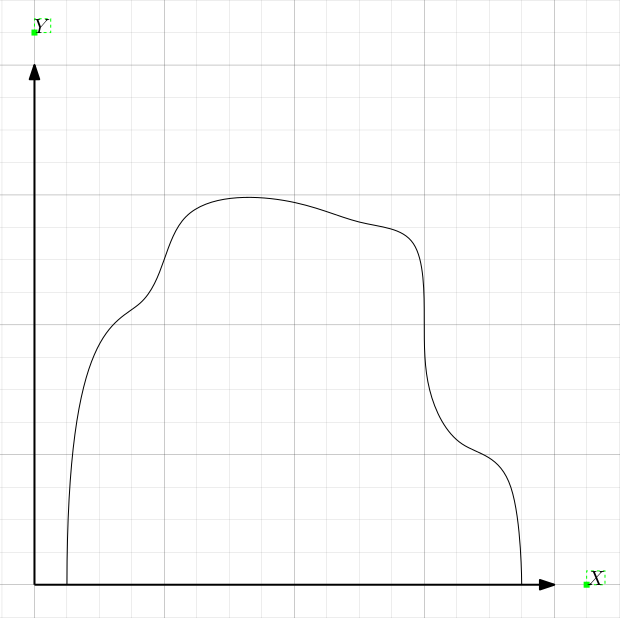
If the function was given to us in closed form, we might have been able to compute the integral using the fundamental theorem of calculus, but that is clearly not of much use to us: our radiance function is not provided in a closed form.
Actually, the situation is even worse. With cubemaps, we have a very limited amount of information about the function. In fact, all we have is a fixed number of samples (texels) on a regularly spaced grid. If a function of a single variable was given to us in the same manner, it would look something like this:
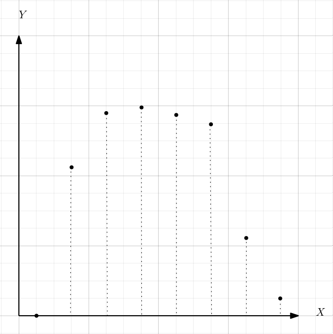
How do we integrate that? We could try Monte-Carlo again, and apply a nearest-neighbor or linear filter to reconstruct values between the samples. However, it is actually sub-optimal for this case. Those readers who are familiar with analysis have probably picked up on the answer by just looking at the image above. That answer is Riemann sums.
The Riemann sum method might be familiar to you from your basic analysis course. You might have used it before for functions of one variable, but it generalizes to higher dimensions:
- split your domain of integration into non-overlapping sections (for functions of one variable those are 1D intervals);
- for each section:
- pick any point within that section and evaluate your function at that point;
- multiply the result obtained above by the "measure" of the section (for functions of one variable it's the length of the interval, for functions defined on a 2D domain it may be the area)
- add up the results for each section and that's your approximation of the integral
This is pretty simple for functions of one variable, but our case is a bit more complicated. Our domain of integration is a sphere. We split it into sections by projecting each cubemap texel onto the sphere: each projected surface patch is its own "section".
But unlike the 1D case, computing the areas of those patches isn't completely trivial. Those areas are proportional to the solid angles subtended by the corresponding cubemap texels, and they can vary from patch to patch. Here is a diagram to help visualize the problem:
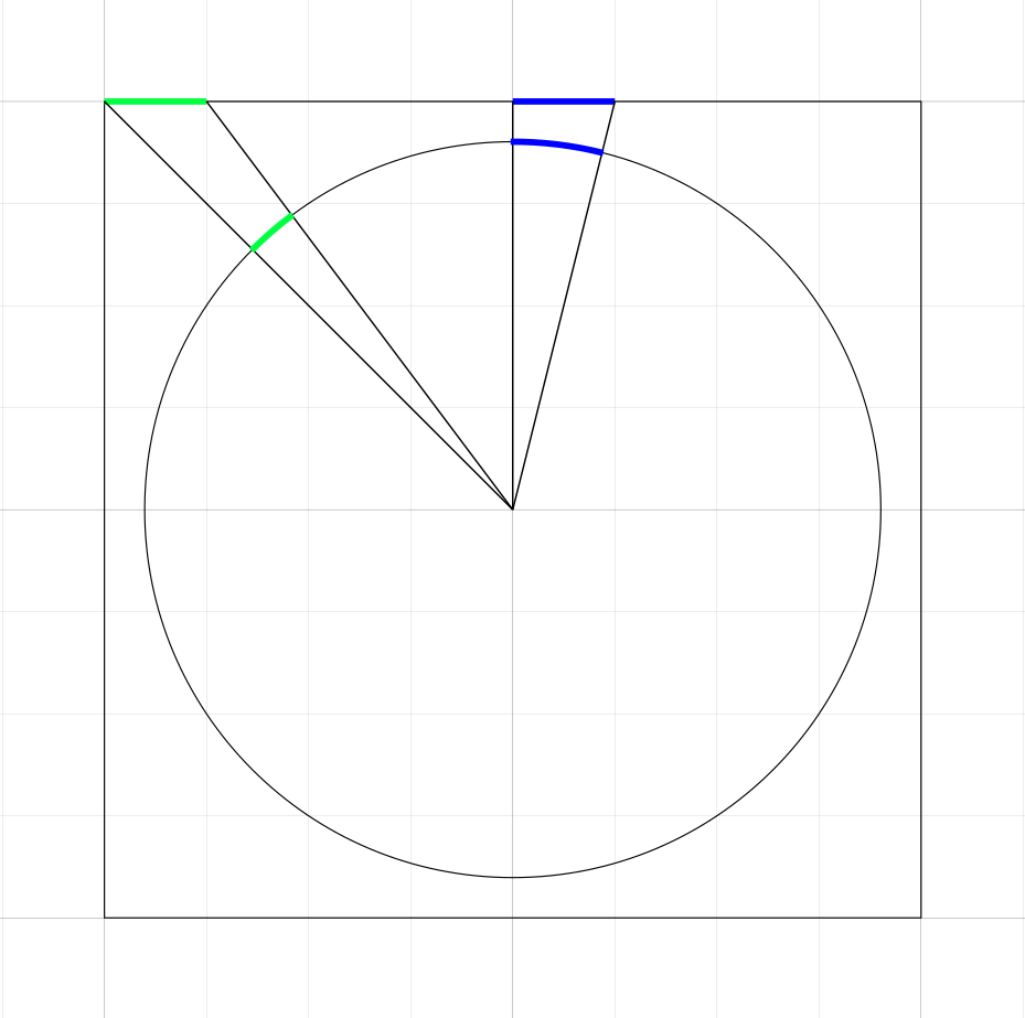
Imagine the sphere being inscribed into the cubemap, and the cubemap texels being projected onto the surface of the sphere. The picture above illustrates that even though the blue and green texels are the same size on the cubemap, the areas of their projections onto the sphere are actually different.
There is actually a relatively simple method for computing the areas of these projections, and it's covered really well in this post by Rory Driscoll, so I won't be re-explaining it here.
There is an even simpler method to estimate this area used in Peter-Pike Sloan's Stupid Spherical Harmonic Tricks paper, but it's less precise.
So, given all of the above, our plan of attack is:
- assume the cubemap fits into a (-1,-1,-1) - (1, 1, 1) cube;
- assume our area of integration - a unit sphere - is inscribed into that cube;
-
For each texel of each cubemap face:
- obtain the value of the texel $T(p)$;
- project the texel center $p$ onto the surface of the sphere to obtain point $p'$;
- evaluate the spherical harmonic basis functions at that point: $y_0^0(p'), ... y_{\ell}^\ell(p')$;
- compute the area of the projected patch $S_{p'}$;
- compute the products $t_0^0 = T(p)y_0^0(p')S_{p'}, ..., t_\ell^\ell = T(p)y_\ell^\ell(p')S_{p'}$ and add them to their corresponding running totals $c_0^0,...,c_\ell^\ell$.
- $c_0^0,...,c_\ell^\ell$ now contain the SH coefficients we sought to find.
When translated to Javascript this recipe looks like the following:
const CUBE_DIM = 128;
const TEXEL_SIZE = 1.0 / CUBE_DIM; // texel size in UV space.
const HALF_TEXEL_SIZE = 0.5 * TEXEL_SIZE;

// Projects a given cube map to spherical harmonics of degrees up to
// and including maxDegree.
function projectCubemapToSH(cube, maxDegree, gammaCorrection = false) {
  // Computes the solid angle subtended by the given texel.
  // Derivation:
  // https://www.rorydriscoll.com/2012/01/15/cubemap-texel-solid-angle/
  function calcTexelWeight(x,y) {
    const x0 = x - TEXEL_SIZE;
    const y0 = y - TEXEL_SIZE;
    const x1 = x + TEXEL_SIZE;
    const y1 = y + TEXEL_SIZE;
    function areaElement(a, b) {
      return Math.atan2(a*b, Math.sqrt(a*a + b*b + 1));
    }
    return areaElement(x0, y0) - areaElement(x0, y1) - areaElement(x1, y0)
          + areaElement(x1, y1);
  }

  // We treat each of the red, green and  blue channels as a separate
  // function to approximate.
  // Thus, our output will be three sets of SH coefficients:
  // for red, green and blue respectively.
  var shRgb = [
  [],[],[]
  ];

  for(var face = 0; face < 6; ++face) {
    for (var col = 0; col < CUBE_DIM; ++col) {
      for (var row = 0; row < CUBE_DIM; ++row) {
        const texelColor = cube[face].data.slice(
            4*(col + row * CUBE_DIM),
            4*(col + row * CUBE_DIM) + 4);
        // UV (0,0) is the top-left corner of the image.
        // UV (1,1) is the bottom-right.
        const faceCoords = cubemapFaceCoords(col, row);
        const d = cubemapCoordsToDirection(face, faceCoords);
        const texelWeight = calcTexelWeight(faceCoords[0], faceCoords[1]);
        const sh = evalSHBasis(d, maxDegree, 1);
        const texelColorf_raw = new Float32Array([
          texelColor[0]/255.0,
          texelColor[1]/255.0,
          texelColor[2]/255.0])
        const texelColorf =
          gammaCorrection ? srgbToLinear(texelColorf_raw) : texelColorf_raw;
        const shRed = mulScalarBySHCoeffs(texelWeight * texelColorf[0], sh);
        const shGreen = mulScalarBySHCoeffs(texelWeight * texelColorf[1], sh);
        const shBlue = mulScalarBySHCoeffs(texelWeight * texelColorf[2], sh);
        shRgb[0] = addSHCoeffs(shRgb[0], shRed);
        shRgb[1] = addSHCoeffs(shRgb[1], shGreen);
        shRgb[2] = addSHCoeffs(shRgb[2], shBlue);
      }
    }
  }
  return shRgb;
}
Couple things to note here. First is the `calcTexelWeight` function. As explained earlier, it computes the solid angle subtended by the cubemap texel, and this is very important for our integration to be correct. I do urge you to go and read the post with the explanation of why this weighting function works. I've verified it by checking that all weights sum up to something very close to $4\pi$.
The second point of interest is the "gamma correction" parameter. Usually, if you were to project a cubemap to SH, you would deal with an HDR cubemap that stores actual radiance values (usually generated by your rendering engine). But, in our sample, all cubemap data is stored in SDR images using sRGB encoding. So, I have added the option to gamma-correct the input. It's your bog-standard pow(value, 2.2), so I'm not wasting space on showing it.
Finally, `cubemapFaceCoords` and `cubemapCoordsToDirection` functions exist to calculate a unit vector aimed at the center of a particular cubemap texel. They're important to get right, but not very interesting, so you can look at them by looking at the full sample source code.
The last piece that we need is the actual evaluation of the spherical harmonics representation of a function. Given the spherical harmonics coefficients, how do we obtain the approximated values of our function? It's pretty simple:
// Evaluates the given SH representation of a function projected onto
// l-band basis in the given direction.
function evalSHRepresentation(coeffs, d, l) {
  // evaluate each basis function for the given direction.
  const basis = evalSHBasis(d, l);

  // multiply the values of the basis functions in the given direction
  // with the respective SH coefficients.
  const basis_coefs = coeffs.map(function(c,i) { return c * basis[i]; });

  // add up the results.
  return basis_coefs.reduce(function(a, v) { return a+v; }, 0.0);
}
The sample uses this procedure to convert the SH representation back into a cubemap that can be shown to the user.
Try playing around with this sample a bit. You will notice that it has an mysterious option called "apply deringing". That option will take the whole of the next section to explain...
Spherical Harmonic Artifacts
Up until now we have been pretending that the projection of any arbitrary function onto a finite SH basis is an "approximation" that is useful enough in practice. But, unfortunately, not everything is so easy.
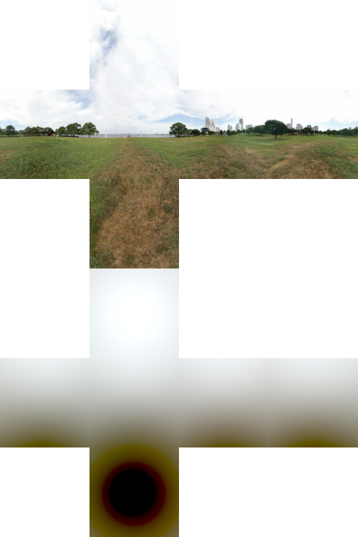
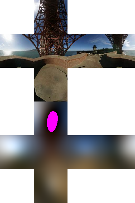
If you look at the Yokohama cubemap at $\ell=1$ with gamma correction on, you will notice the approximation has a strange "hole" in the bottom:
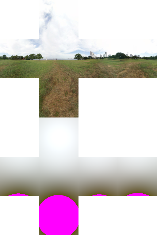
Highlighting negative values reveals something curious: our SH representation evaluates to less than zero in many regions:
Gamma correction makes it worse, but is by no means necessary for these artifacts to appear. For example, the Golden Gate cubemap at $\ell=3$ has negative values without any gamma correction:
So what's going on? Our source cubemap didn't contain any negative values at all, so how can our approximation yield them? And why does gamma correction seem to make the issue worse?
Recall what was said earlier: any continuous real-valued function $f(\theta, \phi)$ defined on the sphere is representable as an infinite sum:
$f(\theta, \phi) = c_{0}^{0}y_{0}^{0}(\theta,\phi) + c_{1}^{-1}y_{1}^{-1}(\theta,\phi) + c_{1}^{0}y_{1}^{0}(\theta,\phi) + c_{1}^{1}y_{1}^{1}(\theta,\phi) + ...$
This is a true mathematical fact. However, when we use spherical harmonics in practice, we kind of handwave away two really important conditions: first, instead of using an infinite basis, we use a finite subset of it. Second, we often try to project weird, potentially discontinuous functions (like our cubemaps).
Mathematics doesn't tolerate such transgressions. It punishes us with horrible artifacts called "ringing" or "Gibbs phenomena". When that happens (usually when the input function has rapid changes/discontinuities), our "approximation" ends up with dramatic overshoot/undershoot around the problematic regions. We could get negative values when evaluating our approximation, even if the function we were trying to approximate is strictly positive! As you might imagine, this is quite catastrophic for lighting, because there's no such thing as "negative" light.
This also explains why turning on gamma correction makes the issue worse: linearizing the values makes the difference between the darks and the highlights more dramatic, making the function more prone to ringing.
To fix this, our first instinct might be to pile on even more frequency bands. It quickly becomes impractical though as the number of required coefficients grows quadratically. More importantly, a discontinuous function is like a signal that has an infinite frequency, so no matter how many frequency bands you add, you will never guarantee that your result will be free of negative values.
The usual way to deal with this problem (suggested in Sloan's paper) is to multiply the coefficients of the projection by another set of coefficients that taper off to zero as the corresponding degree $\ell$ increases. The paper calls this procedure "windowing". The function that defines how the windowing coefficients drop off with $\ell$ is called the "windowing function".
The windowing function used in this sample is sinc:
$ w(\ell)= \begin{cases} 1, \ell = 0 \\ (\frac{\sin\frac{\pi\ell}{q}}{\frac{\pi\ell}{q}})^p, \ell > 0 \end{cases} $
Where $q$ is a parameter that controls how fast the windowing coefficients drop off to 0 as $\ell$ grows, while $p$ is a parameter that controls how "aggressively" deringing is applied (more on that later).
But why does this work at all? Well, spherical harmonics is something that in digital signal processing is called a "frequency domain representation". That is, it represents an arbitrary signal as a weighted sum of known signals of different frequencies - the higher the degree $\ell$ the higher the frequency.
Applying the windowing function can be seen as gradually reducing the influence of higher frequencies on the output - that is, applying a kind of low-pass filter. Which is equivalent to just "blurring" the input signal. Of course, by blurring the input signal we will reduce rapid changes and discontinuities - at the expense of getting a less detailed result.
So, this method of deringing is really just a way to "blur" the input signal in an attempt to get rid of the discontinuities that cause the ringing artifacts. The $q$ parameter of our windowing function controls the "width" of the blur (i.e. which frequencies should be cut off), while the $p$ parameter effectively controls how many times the blur is applied - sometimes, applying it just once doesn't get rid of all the negative values.
Case Study: Projecting Irradiance to Spherical Harmonics
For our next example, we will look at how irradiance is projected to spherical harmonics. We will refer to the talk from GDC 2018 by Yuriy O'Donnel, "Precomputed Global Illumination in Frostbite", more specifically the section dedicated to diffuse lighting in lightmaps.
Spherical Harmonics and Lightmaps
As you might already know, lightmaps are special textures that store the amount of light arriving at each point on the surface of a given scene. "Amount of light" is a bit of a wishy-washy term. Most often, lightmaps store some approximation of irradiance at a point, i.e. this integral:
$E(p) = \int L_i(\vec{\omega}, p) \max(0, (\vec{\omega} \cdot \vec{n})) d\vec{\omega}$
where $p$ is the point on the surface, $L_i(\vec{\omega}, p)$ is the light arriving at $p$ from direction $\vec{\omega}$ and $\vec{n}$ is the surface normal at the point $p$.
Indeed, that is the quantity that Frostbite's lightmap implementation from the talk uses:
We use low-order L1 spherical harmonics to store irradiance data in our lightmaps.
But wait, how exactly is irradiance related to spherical harmonics?
If we fix the surface point $p$, the irradiance can also be thought of as a function of the surface normal at that point:
$E(\vec{n}) = \int L_i(\vec{\omega}, p) \max(0, (\vec{\omega} \cdot \vec{n})) d\vec{\omega}$
That is a function defined on the surface of a sphere. What Frostbite's presentation is saying is that they are storing the spherical harmonics coefficients of that function (up to and including band $\ell=1$), and evaluate it at runtime using the actual normal used for shading. But what is the point of storing the irradiance as a function of the surface normal?
When your meshes use normal maps, you want baked lighting to capture the detail expressed by those normal maps. If you just store some value, the baked lighting will look flat. The image below shows exactly this: the area in shadow receives indirect light thanks to the lightmap, but any variation due to the normal map is completely lost.
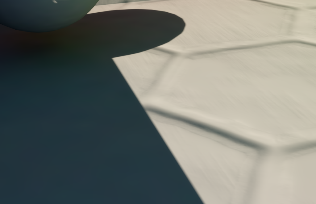 Image credit: Matt Pettineo
You might say: well, this is really easy to solve - just include the surface normal extracted from the normal map in your offline calculations! While this could work theoretically (even though it would prevent you from being able to perturb the shading normal at runtime), it has a pretty big drawback: each texel of your light map would have to correspond to one texel of the normal map.
Yes, your lightmaps would have more detail, but they would be larger (and bake slower). Instead, you can generate the lightmap with lower resolution, but make each texel contain the approximation of a function that tells us what the irradiance at that point would be if the surface normal at that point was oriented in a particular way.
So, by making the lightmap store irradiance as a function of the surface normal we:
- allow the baked lighting to react to the content of the normal map;
- allow perturbing the normals at runtime;
- reduce required space and bake times
Spherical Harmonics and Convolution
Here is how the presentation describes the process of computing the irradiance SH representation:
For rendering, we need to compute the amount of light that falls on a surface with a particular normal from all directions on a hemisphere around it. In other words, we need to compute irradiance at a particular point on the geometry surface.
This is achived by convolving the radiance function in SH form with [...] clamped cosine.
SH is a frequency-space representation of a signal and a convolution in this form is simple per-component multiplcation of the SH basis factors.
To understand this, we need to look at another mathematical concept - convolution - and examine how it interacts with spherical harmonics. Bear with me for a few paragraphs, and it will become obvious how this is connected with irradiance.
You might already be familiar with the idea of convolution from image processing, where it means "sliding" a matrix of coefficients ("filter") across an image, while multiplying the values from the image with the corresponding values from the filter and summing everything up.
This concept can be generalized for the world of functions. For functions $f$ and $g$ defined in Cartesian coordinates, the definition of the convolution operation $(f*g)$ is straightforward:
$(f*g)(t) = \int f(\tau)g(t-\tau)d\tau$
As you can see, convolution in Cartesian coordinates amounts to "sliding" one function over the other, multiplying the functions and integrating the result. In other words, to evaluate the convolution at point $t$, we "center" one of the functions (which is called the "kernel", in the above definition $g$ plays that role) around $t$ and integrate the product of the centered kernel with the other function.
However, in our case, we are dealing with functions defined on the sphere, so this definition of convolution doesn't quite work. We need the functions to "slide" on the sphere, so this definition has to be modified a bit.
Let's say we have two functions defined on the surface of the sphere, $f(\vec{w})$ and $g(\vec{w})$. Furthermore, let's define $\rho_t(g)$ as the result of "rotating" the function $g$ such that its "north pole" aligns with the direction $t$. The convolution of $f$ and $g$ is then defined as:
$( f*g)(t) = \langle f, \rho_t(g) \rangle = \int f(\omega)\rho_t(g(\omega)) d\omega $
The rotation operation in this case plays the role of centering that we used for the Cartesian case.
Finally, let's look at an interesting property of spherical harmonics related to convolution.
Let's say that $f_\ell^m$ are the SH coefficients corresponding to the function $f$. Further, let's assume $h$ is a function that is rotationally symmetrical around $Z$ axis (i.e. it doesn't change value when the azimuthal angle changes). It turns out that the SH coefficients of the convolution $f*h$ can be found using the formula:
$(f*h)_\ell^m = \sqrt{\frac{4\pi}{2\ell+1}}f_\ell^m h_\ell^0$
Why do we care about convolutions and finding their SH coefficients? Take another look at the irradiance integral:
$ E(\vec{n}) = \int L_i(\vec{\omega}, p) \max(0, (\vec{\omega} \cdot \vec{n})) d\vec{\omega} $
$(\vec{\omega} \cdot \vec{n})$ is just $g(\theta, \phi) = \cos{\theta}$ rotated so that its "north pole" aligns with the surface normal $\vec{n}$. Once you understand that, it immediately becomes obvious that irradiance is the result of convolving the radiance $L_i$ with the cosine (or, "clamped" cosine, to be precise).
Finding the SH Coefficients for Irradiance
We know how to obtain SH coefficients for radiance. The "clamped cosine" function we saw earlier has well-known SH coefficients. You can find them in the paper by Ramamoorthi and Hanrahan, "An Efficient Representation of Irradiance Environment Maps":
$A_0 = \frac{\sqrt\pi}{2}, A_1 = \sqrt{\frac{\pi}{3}}$
So is that it, we're done? Just project the radiance onto spherical harmonic functions with $\ell = 0, 1$, multiply the coefficients in band $\ell=0$ by $A_0$ and coefficients in band $\ell=1$ by $A_1$ and call it a day?
Well, that would definitely work, but we can improve on it a bit. The Frostbite presentation shows us a really neat trick that allows the evaluation step to be simplified. Recall that in order to compute the SH coefficients of a convolution we have to do this:
$(f*h)_\ell^m = \sqrt{\frac{4\pi}{2\ell+1}}f_\ell^m h_\ell^0$
In case of irradiance, our functions are radiance $L_i$ and the clamped cosine, which we'll denote $A$:
$(L_i*A)_\ell^m = \sqrt{\frac{4\pi}{2\ell+1}}L_\ell^m A_\ell^0$
Let's try doing some simplifications for $(L_i*A)_0^0$. Given that $A_0 = \frac{\sqrt{\pi}}{2}$, we have:
$(L_i*A)_0^0 = \sqrt{4\pi}L_0^0 \frac{\sqrt{\pi}}{2} = \pi L_0^0$
Because $L_0^0$ is a sum of products of $y_0^0$ with various values of radiance, we can pull out the constant term: $L_0^0 = \frac{1}{2\sqrt{\pi}} (...)$. Therefore:
$(L_i*A)_0^0 = \pi\frac{1}{2\sqrt{\pi}} (...) = \frac{\sqrt{\pi}}{2} (...)$
But we know that during evaluation at runtime, we will have to multiply this value with $y_0^0$ again, which has a constant factor. So why not fold that constant factor $\frac{1}{2\sqrt{\pi}}$ into the irradiance computation?
$\frac{1}{2\sqrt{\pi}} (L_i*A)_0^0 = \frac{1}{2\sqrt{\pi}} \frac{\sqrt{\pi}}{2} (...) = \frac{1}{4}(...)$
You can look in the PDF for the other derivations, but the upshot is: we can combine the radiance projection, convolution and partial evaluation into one short function:
SHL1 shEvaluateDiffuseL1(vec3 p)
{
  float AY0 = 0.25f;
  float AY1 = 0.50f;
  SHL1 sh;
  sh[0] = AY0;
  sh[1] = AY1 * p.y;
  sh[2] = AY1 * p.z;
  sh[3] = AY1 * p.x;
  return sh;
}
The value returned by that function is what gets stored in the lightmap, and the really neat part is that to evaluate it for a given normal it's just a dot product with the normal! All the other computations have already been done at the baking step.
Conclusions and Further Reading
This post could have covered more topics, but my intention is to give readers the vocabulary and knowledge necessary to understand writings published by some very smart people. So, I'd like to conclude with a few recommendations on where to proceed from here.
To start with:
- Peter-Pike Sloan, "Stupid Spherical Harmonics Tricks", which has been mentioned multiple times here.
- Robin Green, "Spherical Harmonic Lighting: The Gritty Details"
- Ravi Ramamoorthi and Pat Hanrahan, "An Efficient Representation for Irradiance Environment Maps"
Deringing spherical harmonics is a much more challenging problem than this post might have made it sound. Peter-Pike Sloan's "Deringing Spherical Harmonics" paper goes in-depth on a more principled approach to deringing that attempts to preserve as much detail as possible while fully avoiding negative values in the projected irradiance.
Two posts on Graham Hazel's blog are well worth a read:
These together explain how it's possible to avoid negative values for L1 spherical harmonics by just tweaking the definitions a bit (sadly, doesn't work for higher degrees). The Frostbite talk that we had looked at mentions using these techniques.
Spherical harmonics are by no means the only way of representing lighting information. A couple alternatives:
- Chris Green, "Efficient Self-Shadowed Radiosity Normal Mapping " (HL2)
- Ralf Habel and Michael Wimmer , "Efficient Irradiance Normal Mapping" (H-Basis)
- This wonderful series by Matt Pettineo is a great resource that explains some general ideas about lightmapping and goes in-depth about spherical Gaussians, which are another lighting representation.
I hope you enjoyed this post. If you've found any errors, let me know by e-mailing nicebyte at gpfault.net.
Like this post? Follow me on bluesky for more!